


Control of radioactive fallout from the Chernobyl accident
based on cross-checks from the IRSN simulation1,
of the official ATLAS2 of Cs137 surface concentrations,
and recorded daily rainfall by weather stations at airfields and airports3.
Yves Lenoir4
Introduction
Few people are not familiar with the map of radioactive fallout from the explosion of Block 4 of the Chernobyl atomic power station on the night of 26 April 1986. From the very first critical examination, the question arises of a reality, marvellous if one thinks about it: not a single large city in the republic of Belarus, the Baltic States, Russia and the Ukraine has suffered significant fallout! The quarter-hour by quarter-hour reconstitution of the atmospheric transport of discharges from the plant during the two weeks from 26 April to 9 May 1986, carried out by the IRSN in 2005, provides an initial trivial answer: where the density of radioactive plumes remained low, the fallout was low, if not zero. For Moscow, St. Petersburg, Riga, Tallinn, etc., the results were similar. On the other hand, the very low levels of contamination around Kiev and Bryansk do not seem to be the result of a natural process.
The challenge of the cross-analysis undertaken here following this empirical observation is to test the hypothesis of the non-natural character of the meteorological phenomena at work before and during the passage of radioactive plumes over these cities, and perhaps others as well. The figures will speak for themselves.
It is also striking that there was almost no fallout on the territory of Poland and the Baltic States, even though they were overflown for several days by particularly dense plumes. Only the lack of rainfall during these critical days can explain why they were spared, which will have to be verified with impartial figures.
Method
1. The rainfall issue
Dry deposits are known to be 1/100th or less lower than wet deposits. This means, for example, that if it has rained for three hours during the passage of the cloud, the dry contributions before and after this rainy episode will have little influence on the quantity of radionuclides deposited on the ground during this nine-hour interval - accepting the hypothesis of relatively slow variations in the radioactive density of the plume from a certain distance from the source of the releases, the accident reactor.
Daily rainfall between 26 April and 9 May 1986 is therefore the crucial variable. The most reliable data are those routinely collected and archived over the past 100 years by meteorological stations at aerodromes and airports. They can be found on two sites, cf. [3]; sometimes a missing station on one site is archived on the other, which ensures the completeness of the data. However, the small number (19) of airports and aerodromes on the territory of Belarus led us to search for other stations presenting the meteorological data recorded during the radiological crisis. Informed, the Director of Belrad, Alexey Nesterenko, sent us an official document which adds about thirty stations to those of the airports; it provides, among other maps and explanations, the heights of the daily rainfall that occurred between 26 April and 10 May 1986.
It will be seen that the rainfall figures appearing in the official ATLAS referenced in [2] are unreliable - or even absent (Norway), or fanciful (Poland)5. However, so that this assessment is not considered as an a priori judgment, two parallel processing of the data was carried out, one using the rainfall heights recorded by the airport stations and the other using the heights extracted from the daily rainfall maps of the ATLAS. The inconsistencies that were obvious at the time became numerical in nature.
The working base is made up of the three Baltic countries, the Scandinavian countries outside Denmark, Poland, Belarus, Ukraine and Russia in Europe. The sample base consists of 380 meteorological stations selected from more than 500, distributed in the order of the first plumes:
- Belarus, 51
- Lithuania, 15
- Latvia, 9
- Estonia, 9
- Sweden, 74
- Norway, 34
- Finland, 27
- Poland, 58
- Ukrainea, 49
- Russia, 54
- Total 380
Each station is indexed by a number.
2. The establishment of the maps
This involves placing the indexes of the 380 stations on maps drawn up with different projections.
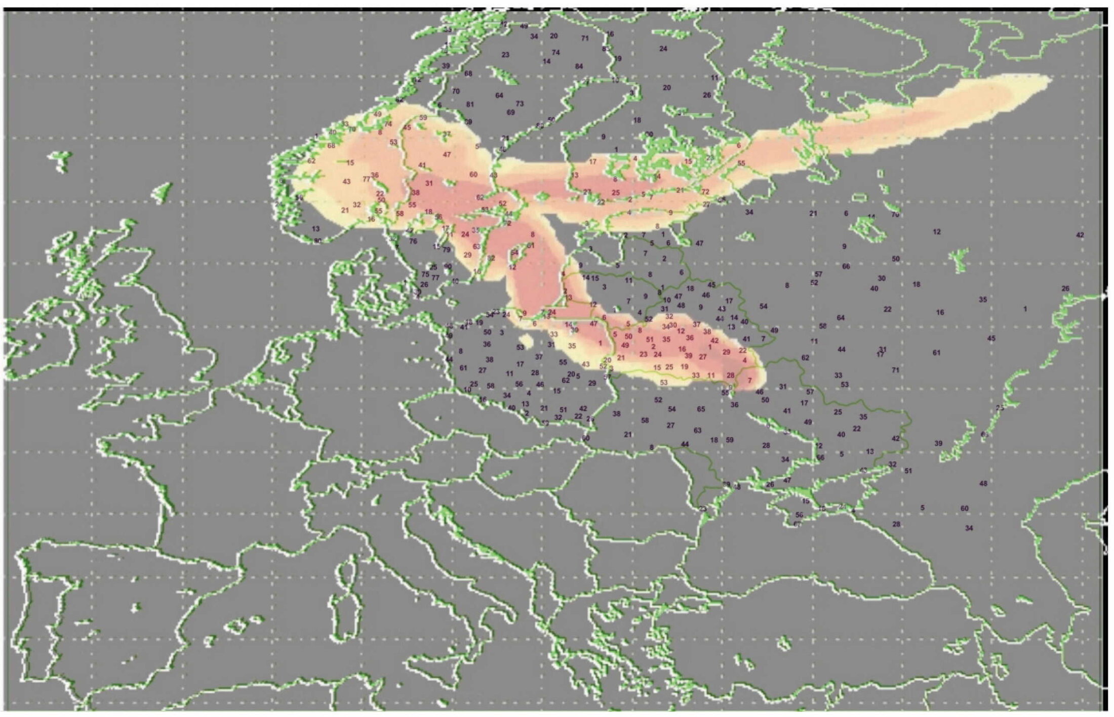
The one adopted by IRSN is a Mercator. Starting from a screenshot of the initial map, just before the explosion, the indexes were placed one after the other, with the help of partial maps and/or the longitudes and latitudes of the stations. Once the station map was created, it was printed on a layer that was then applied to the screen in such a way that its contours coincided with those of the IRSN map.
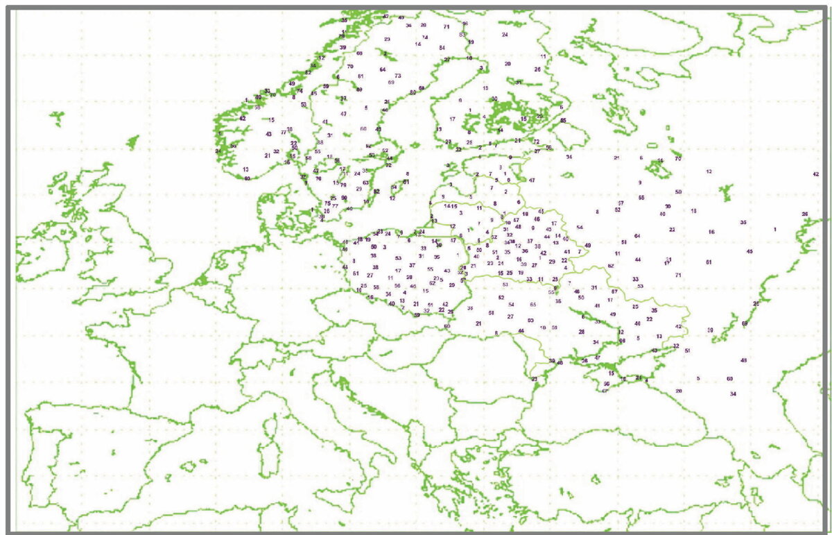
Agrandissement : Illustration 1
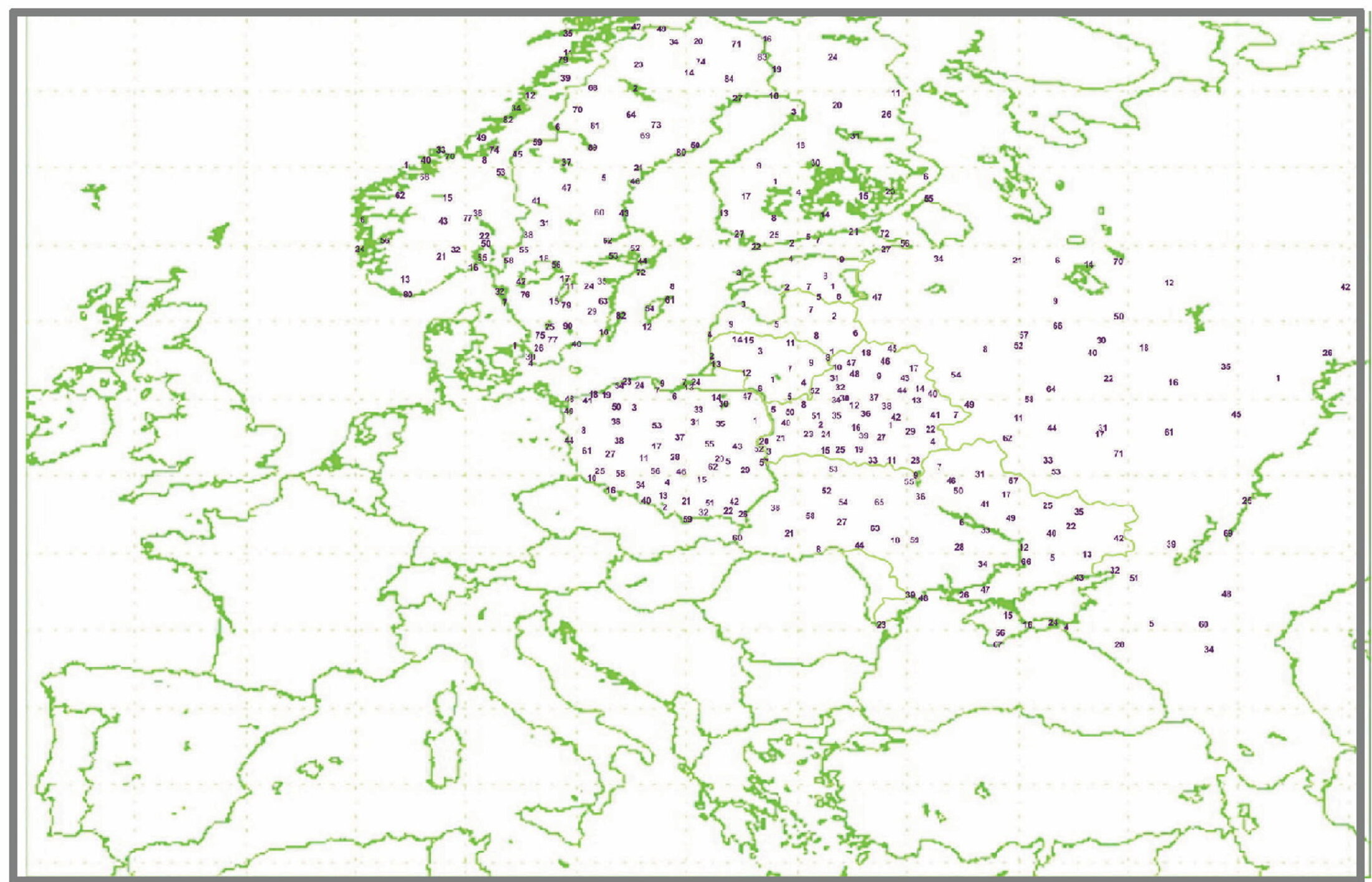
Layer to the proportions of the IRSN map with the 380 meteorological stations
Equivalent procedures were applied to the fallout and rainfall maps presented in the official ATLAS. Examples below for Belarus – soil contamination and rainfall of 28 April 1986:
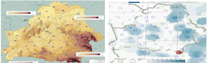
Agrandissement : Illustration 2
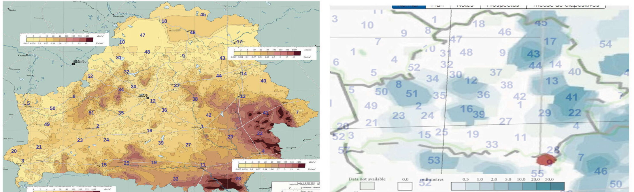
Cs137 fallout on Belarus Rainfall of 28 April 1986 on Belarus
3. Procedure for measuring the density of radioactive plumes
The simulation is progressed in 3-hour intervals (8 readings per day). The colour of the indexes is clearly distinguishable from those which parameterise the density of the plume as can be seen on the capture below corresponding to the situation on 28 April 1986 at about 13h:

Agrandissement : Illustration 3
General situation on 28 April 1986 around 1 p.m. (IRSN simulation with superimposed indexes)
Colour coding, such as that used in the ATLAS for soil contamination, follows a logarithmic scale of base 10, each colour range thus covering an order of magnitude of the density, expressed in Bq/m3, of the air contamination between 0 and 10 m above the ground. There are six colour ranges, from 0.01-0.1 Bq/m3 to 100 - 1,000 Bq/m3 for the first five, from yellow to dark brown, plus black for densities above 1,000 Bq/m3.
The readings are taken in order of magnitude with the upper value of each interval covered by a colour. The value 0.1 Bq/m3 is not recorded as it is completely negligible. This procedure leads to an overall estimate by excess. The approximation will be partly compensated by an equivalent choice for the soil contamination values in kBq/m2 taken from the ATLAS maps. It is assumed that neither the validity of the calculation of the average coefficients for 112 three-hourly readings per station and 380 stations, nor the validity of the characterisation of possible abnormal deviations are qualitatively affected by this way of processing the data.

Agrandissement : Illustration 4
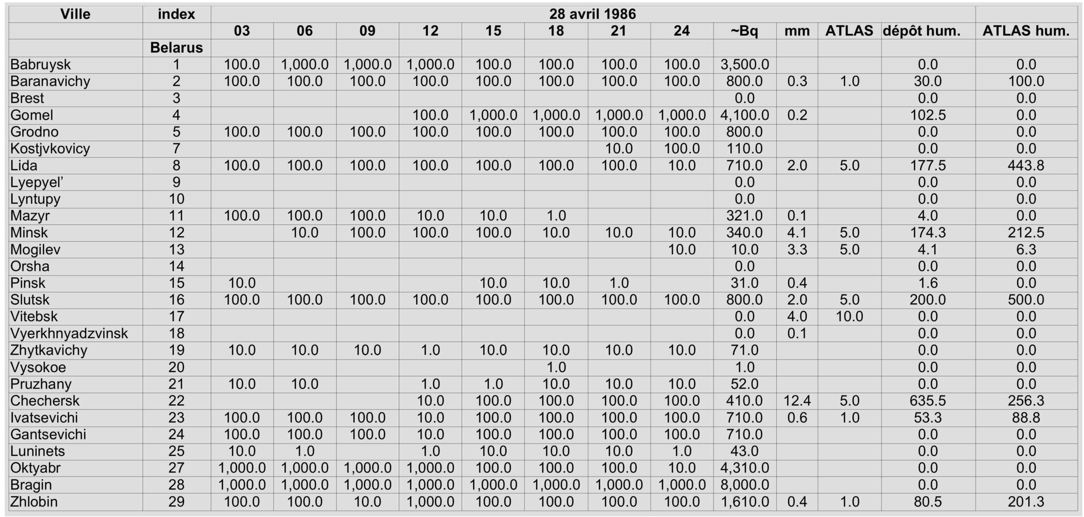
Extract from the general table of cross-analysis of data (Belarus, first 27 lines, 28 April 1986)
- the sum of the 8 densities recorded during the day is entered in the ~Bq column;
- the precipitation values provided by the airport archives are entered in the mm column;
- those taken from ATLAS maps are entered in theATLAS column, also expressed in mm;
- the figures in the hum. deposition column are obtained by dividing by 8 the product ~Bq x mm;
- those in the ATLAS hum. column are obtained by dividing by 8 the product ~Bq x ATLAS.
4. Treatments carried out on all the data collected
4.1 Firstly, the calculations are based on the cumulated data from stations that did not receive rain during the period from 26 April to 9 May; this gives a figure for the relative intensity of dry deposition:
- the ratio between the deposition given by ATLAS and the cumulative total Bq of the 14 values in the ~Bq columns;
- stations where the deposit is less than or equal to 2 kBq/m2 are eliminated because this value, which is recorded in excess in the 1 to 2 kBq/m2 colour range, essentially corresponds to the legacy left by the fallout from atmospheric atomic explosions between 1945 and 1984 (the year of the last Chinese air tests);
- using the two selection rules above, the ratio is established between 100 times the sum of the deposits around these stations and that of the total Bq accumulations for these same stations; this gives the average coefficient of dry deposition, i.e. Ds/Ns = 0.0087 (multiplied by 100 so as not to have minute values).
4.2 The next step is to determine the average wet deposition coefficient from calculations made on the data from each station that received rain:
- The daily records for each station distinguish between dry deposition on rainless days and wet deposition on rainy days;
- We therefore have two distinct totals, that of the densities of "dry" plumes and its equivalent for "wet" plumes;
- from the surface deposits taken from the ATLAS maps, a quantity equal to the "dry" total divided by 100 and multiplied by Ds/Ns is then subtracted;
- the result corresponds roughly to the share of contamination deposited by the "wet" plumes.
As for the treatment of dry deposits, stations where the deposit is less than or equal to 2 kBq/m2 are excluded.
The results take the form of the partial table below:
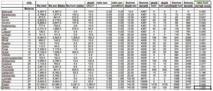
Agrandissement : Illustration 5
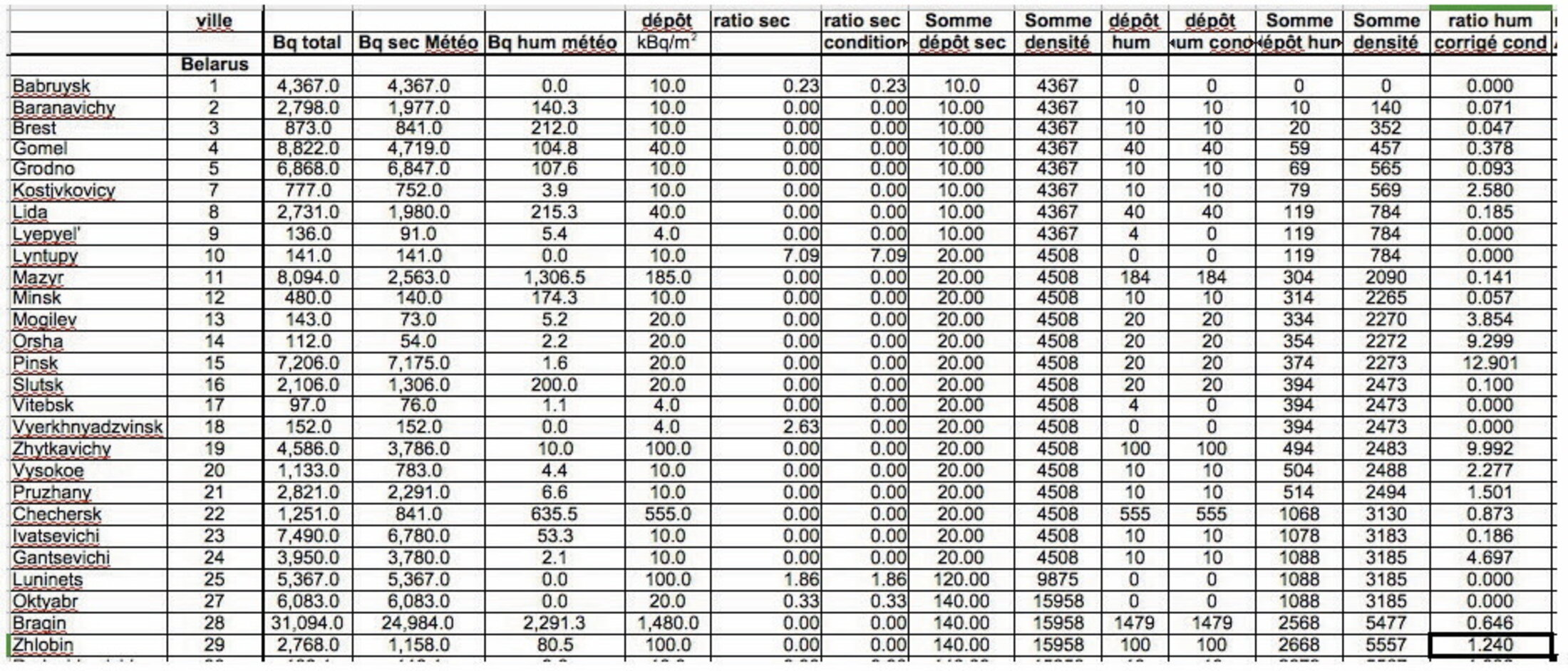
Extract from the general table of cross-analysis of data (Belarus, first 27 lines)
As for dry deposits, the ratio between the Sum of wet deposits and the Sum of wet plume density is calculated. This gives the average wet deposition coefficient:
Dh/Nh = 0.4526 which will be used for comparisons with the relative coefficients at each station for the entire period from 26 April to 09 May 1986 (last column of the above table).
4.3. The origin of the rainfall according to ATLAS seems to be more the result of model estimation than of the collection of data recorded by meteorological stations. The main discrepancies are quantified below:
- the dry deposition coefficient would be 33% higher: Ds/Ns [ATLAS] = 0.0116:
- while the average deposition of the stations in Belarus and Ukraine would be 97.3 and 36.5 kBq/m2, respectively, calculated with wet deposition according to ATLAS, the average deposition around the Polish stations would be 44.4 kBq/m2, i.e. 7 times the 6.4 kBq/m2 of that of the actual measurements;
- except for the border area with Sweden, the precipitation maps that ATLAS has drawn up for Norway are blank. In reality, out of the 34 stations selected, 23 received rainfall between 26 April and 9 May 1986 (for seven of them some information is missing). According to ATLAS, only one station received rain.
This critical evaluation of the differences between the rainfall data provided by ATLAS and the routine readings of aerodromes and airports leads to the rejection of the model with which the authors of ATLAS drew up their rainfall maps.
Analysis and interpretation of the results
1. A contingent calculation process
Numerous approximations affect the readings of the density values of radioactive plumes and Cs137 deposits, as has been recognised from the outset above. Some discrepancies are therefore to be expected between the measured deposition values and those deduced from the sum of the products of dry and wet accumulations by the mean coefficients Ds/Ns and Dh/Nh.
Furthermore, IRSN's simulation is based on a transport and deposition model governed entirely by natural phenomena. If meteorological monitoring techniques have been implemented on a large scale, the systematic treatment described above will reveal significant discrepancies, by default or by excess: by default in the sense that the deposits in protected areas will be much lower than the calculated deposits; by excess where these techniques will have purged the plumes of their radioactive content.
Finally, in view of the high sensitivity of the fallout to precipitation, the sixteen stations for which the meteorological archives were deficient during the period from 26 April to 9 May 1986, and the four Russian stations located outside the ATLAS contamination maps, were eliminated from the analysis of the survey work detailed above. The analysis therefore covers the data from 360 meteorological stations, the radioactive deposits in their vicinity and the cumulative densities of the radioactive plumes that swept over them during these fourteen days.
2. Analysis of the quality of the IRSN simulation
- The first phase of the analysis concerns the comparison between the accumulation of deposits evaluated according to ATLAS maps and that calculated using average coefficients Ds/Ns and Dh/Nh;
- the former is 11,029 against 13,630 for the latter;
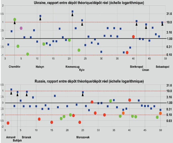
- the second phase consisted in establishing for each of the ten countries considered a graph of the logarithms of the reconstituted deposition / real deposition ratios for each station (numbered in this case according to a continuous index);
- the use of logarithms gives the right visual perspective: for example, a difference of a factor of ten is represented by 1 in one direction and -1 in the other, which means that the graph is, apart from horizontal symmetry, indifferent to the assignment of the numerator and denominator of the ratio.
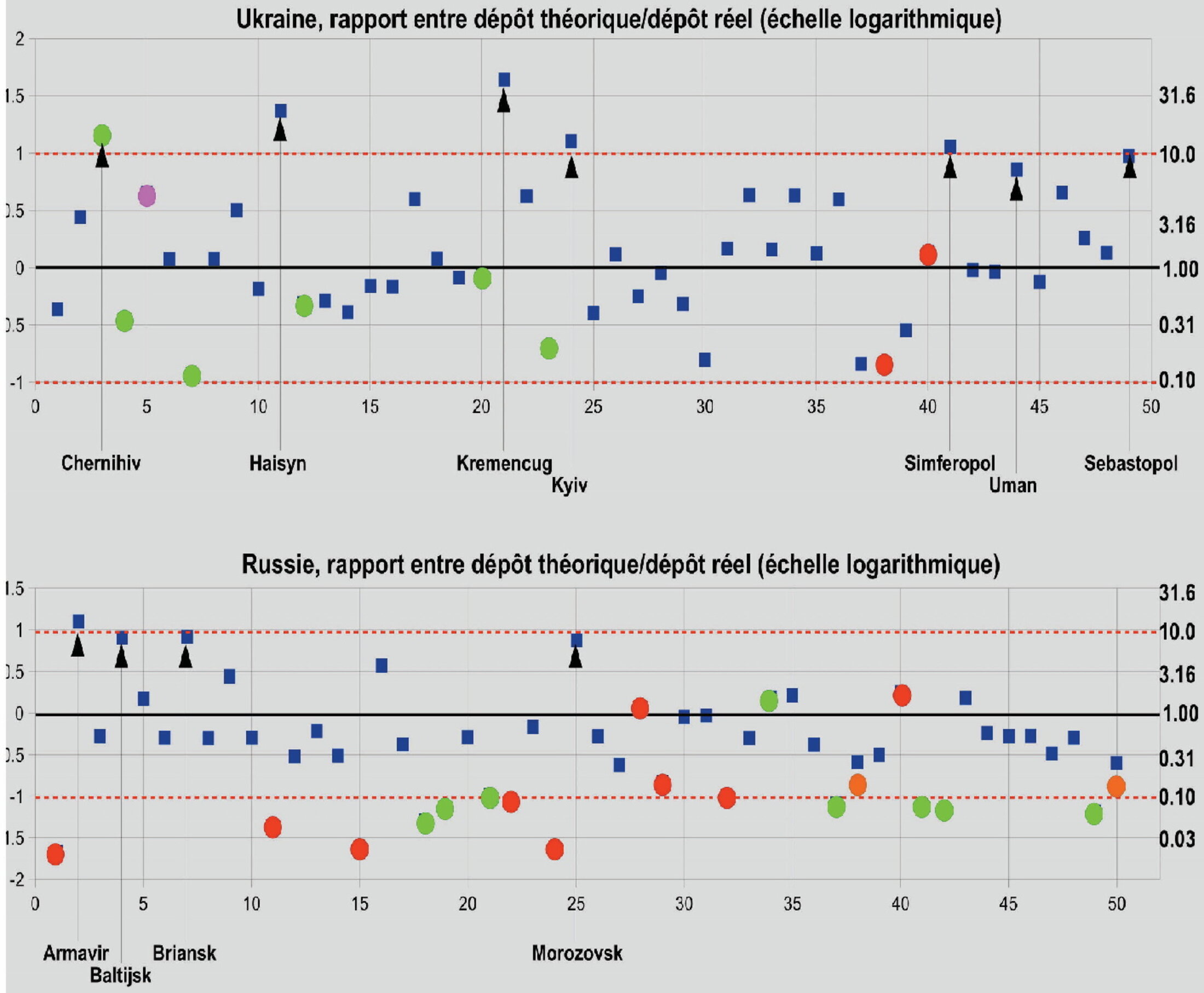
- Example of graphs for Ukraine and Russia:
Agrandissement : Illustration 7
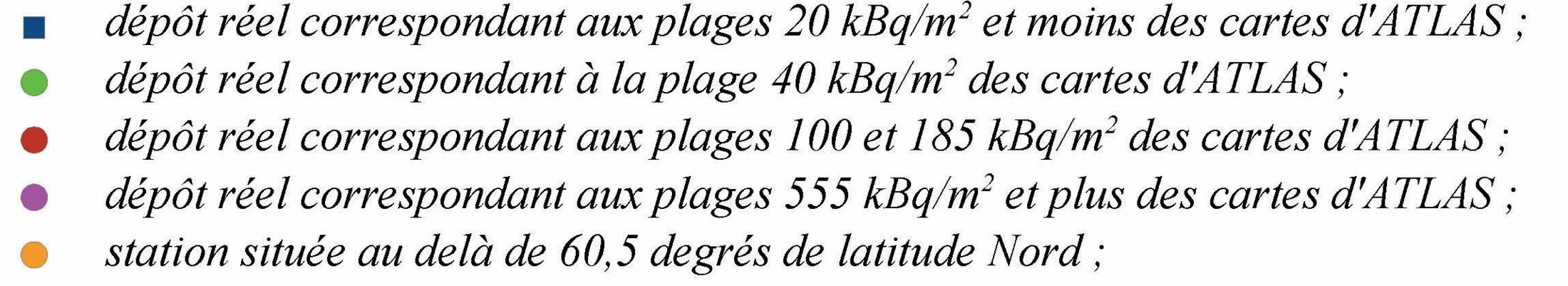
Symbol legend:
- on the x-axis, the continuous index of the selected weather stations;
- left scale: logarithmic value of the ratio [theoretical deposition / actual deposition];
- right scale: arithmetic value of the ratio [theoretical deposition/actual deposition];
equality between theoretical and real deposition;
ordinates corresponding to a difference of one order of magnitude (factor 10) between deposits.
theoretical and actual deposits.

Agrandissement : Illustration 8
- considering that a good concordance is characterised by a ratio between 0.31 and 3.16 (whose logarithms are -0.5 and +0.5), one recognises the excellent coherence of the IRSN simulation; the stations falling within this range are indeed:
• 30 out of 50 for Belarus;
• 28 out of 50 for Russia;
• 29 out of 49 for Ukraine;
• 9 out of 14 for Lithuania;
• 9 out of 9 for Latvia;
• 8 out of 9 for Estonia;
• 35 out of 58 for Poland;
• 44 out of 69 for Sweden;
• 18 out of 27 for Norway;
• 15 out of 25 for Finland.
This is about two thirds of the total results.
The excellence of IRSN's simulation can also be appreciated by comparing it with the one carried out after Fukushima by the team of experts from the Japan Nuclear Energy Safety Organisation (JNES)6:
• firstly, it can be seen that the average of the field measurements (1,889 kBq/m2) is 3.21 times smaller than the calculated values (6,079 kBq/m2).
• in addition, the graph summarising its work shows differences between reality and simulation of between 1000 and 1/1000 (in the interval [-3 ; 3] in logarithmic coordinates). The topography of Japan cannot explain such a dispersion, given that the extension of the territory under consideration does not exceed 100 km:
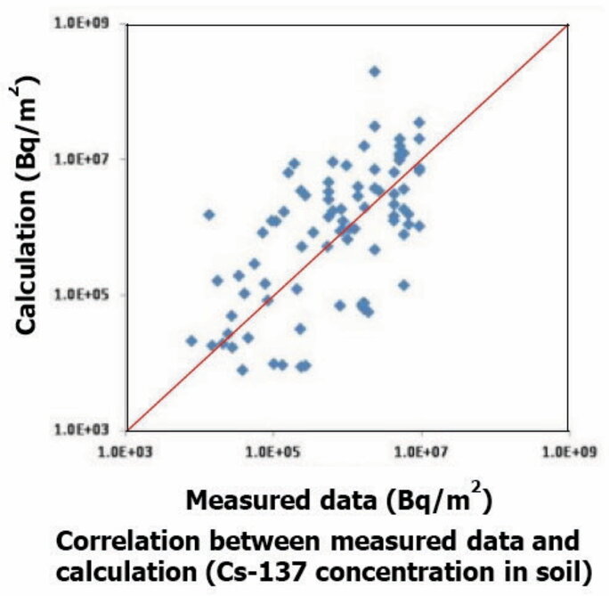
• However, the authors conclude that there is "good agreement between the measurements and the calculated values". It looks more like the result of an overly biased random process drawing numbers between 1 and 1 million!
This is why the low dispersion of the results obtained from the IRSN simulation pleads in favour of the robustness of the method adopted. Consequently, it is reasonable to ask the question of the reasons and causes of the few discrepancies7 characterised by logarithmic values outside the interval [-1 ; +1]. In the first approach, only those for which the measured deposition is greater than or equal to 20 kBq/m2 are considered. The interpretation is then extended to the lower deposition ranges - 2, 4 and 10 kBq/m2.
3. Interpretation of discrepancies between measured and calculated deposits
3.1. We start from the observation that a large city, Kyiv, the capital of Ukraine, has been miraculously preserved from the significant fallout it should have received8 if, from 30 April around 9 a.m. to 5 May at midnight, it had indeed been bathed in a radioactive cloud with a density of between 100 and 1000 Bq/m3, or even more, in Cs137 alone, to which must be added Cs134 in an equivalent quantity, at least three times as much I131, radioactive rare gases, and traces of other radio-elements.
Something unnatural and important had thus happened in the trajectory of the radioactive plume emitted by the burning reactor, for having largely purged the air mass of the radionuclides it was carrying. For the result is there: the soil around Kyiv[36]9 contained at most only 20 kBq/m2 of Cs137.
3.2. The only way to purge a radioactive plume of its contents is to trigger the condensation of the water vapour it contains. The process is known: seeding with silver iodide AgI particles.
The Soviets had a great deal of practice in this matter, acquired during preparatory experiments for the climate war, but also in the meteorological management of major national events, such as the May 1st parade on Red Square, which always had to take place under a radiant sky. One can think that in the framework of the programming of the atomic war they had also carried out tests for the control of "black rains" using the same procedure.
However, the circumstances of Chernobyl posed a complex problem. Radioactive emissions were continuing with alarming intensity. This meant that decisions had to be taken on the basis of random information: from weather forecasts to a week or so ahead. At that time, the modelling of the atmospheric circulation was more or less under control. On the other hand, the forecasts in terms of rainfall remained highly random, even at 24 hours. As we have seen, rain is the key player. It amplifies by a factor of a hundred or more the deposition of radioactive materials on the ground. The difficulty of the exercise is obvious from the meteorological sequence during the crisis:
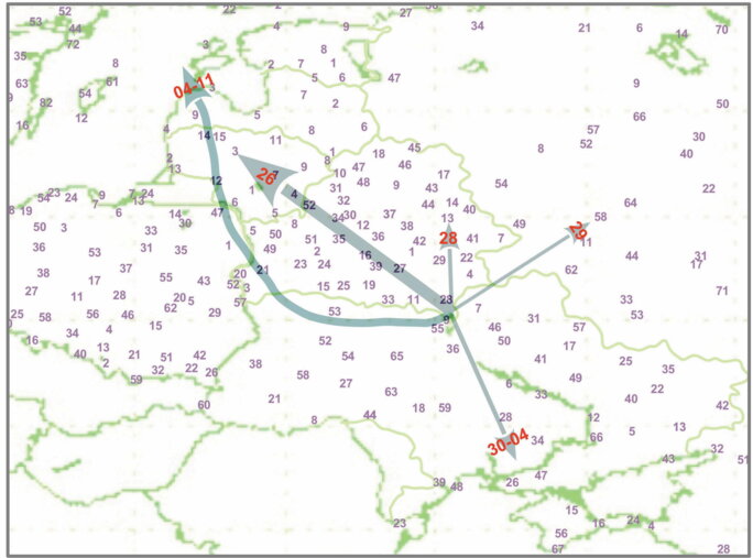
Agrandissement : Illustration 10

Approximate diagram of the trajectories of radioactive plumes
(the thickness of the lines is proportional to their density; the days are written in red)
Thus, the first Chernobyl plume, following the explosion of reactor 4, swept north-westwards over Belarus, Lithuania and Latvia on 26 April in dry weather. The next day, it reached Estonia and Sweden. There was no rain that day over Estonia, but there was some precipitation over part of the Swedish stations, some of which received a "vanguard" plume, albeit still not very rich in radionuclides. But on 27 April, it rained on five stations in Belarus, including 3 mm in the Braghin [28] raion, 40 km north of the power station, leaving a very considerable initial deposit10. In fact, there was no more rainfall in this region until the end of the radioactive discharges on 6 May. The legacy of Chernobyl Belarus was thus already almost entirely attributed there... We can see that the fate of its inhabitants depended on little, 3 mm of rain on 27 April 1986!
3.3. On April 28th around 8 pm, as the radioactivity released since the explosion reached Norway, the wind began to turn over Chernobyl. The region most exposed to the changing weather includes the stations of Gomel [4], Chechersk [22], Braghin [28], Zhlobin [29] and Slavgorod [41]. During this day, it rained a little in Gomel and Zhlobin, and a lot in Chechersk and Slavgorod.
On the 29th, the wind strengthened and blew to the north-east, towards Russia; things became very serious. The weather forecast shows a probable anticyclonic rotation, to the east and then south. In the meantime the plume is under Moscow [40] and, since the day before, threatens Briansk [11] where there are military industrial installations that must be absolutely preserved (manufacture of military trucks and missile launchers). While the weather forecast does not predict rain except around Bryansk, heavy fallout (there can be no more because no plume will then fly over these towns) is taking place in and around Roslavi [49], Smolensk [54], Suhinichi [58], Jeti-Konur [22], and, above all, in the border region with Belarus to the west of the Bryansk oblast in the Novozybkov11 raïon. In Bryansk, despite an accumulation of 3 mm of rain, the fallout is more than eight times less than it should have been. The cloud has been well purged. To all intents and purposes, thanks to the sowing of the Jeti-Konur region, Moscow no longer runs any risk (and in fact has never done so), and for the rest, Bryansk and its immediate surroundings have been spared.
However, everything indicates that, taking advantage of the wet weather, a large purge took place earlier, on the night of the 28th and morning of the 29th, in the region between Chechersk and Slavgorod and above this city. It is thus an already well purged plume that was treated above Russia. As proof, the contaminations measured in Chechersk and Slavgorod12 were respectively13 of 555 and 1,480 kBq/m2, while those affecting the Russian cities14 mentioned above remained between 40 and 100 kBq/m2.
3.4. We now follow the trajectories of the air masses carrying the Chernobyl discharges from the evening of April 28th until late afternoon of May 4th when the wind that has been blowing due south for the past two days begins to turn westward.
In the second part of the day on the 29th and 30th, Chernyhiv [7] is in the densest part of the radioactive cloud. The city will not receive any more radioactivity after 4 May. The actual deposition, 40 kBq/m2, is 16 times lower than that calculated according to the model. A fact that supports a successful purge of the radioactive plume.
The plume then heads due south and widens. Kyiv occupies the core. Two indications of a treatment of the cloud from the start out of the power plant and then beyond the town of Chernobyl [9], 18 km to the south: the latter received "only" 555 kBq/m2 - compared with 2,500 kBq/m2 according to the model; that of Ivankyiv [55], 40 km to the southwest received 185 kBq/m2- compared with 254 kBq/m2 according to the model. But the most determining factor in this case is the huge contamination stain of between 555 and 1480 kBq/m2 covering the territory between Chernobyl city, Ivankyiv and the "Kyiv Sea".
The purged plume will continue on a trajectory that will bend slightly eastward when it reaches the Black Sea coast in the early morning of May 3rd. The protection afforded to the entire region as far as the Crimea is impressive, as evidenced by the relatively low levels of contamination in the settlements along the plume's path from north to south:
- Kyiv [36], capital of Ukraine with 2.8 million inhabitants: 20 kBq/m2 instead of 254 kBq/m2;
- Kremencug [33], a large industrial city, where it rained 25 mm on 2 May: 20 kBq/m2 instead of 880 kBq/m2;
- Uman [59], medium industrial city: 20 kBq/m2 instead of 140 kBq/m2;
- Haisyn [18], small town: 20 kBq/m2 instead of 470 kBq/m2;
- Simferopol [56], large city with high-tech industries, where it rained on May 3 and 4: 20 kBq/m2 instead of 230 kBq/m2;
- Sebastopol [67], a large naval base where it rained on the 3rd and especially the 4th of May (77 mm): 20 kBq/m2 instead of 190 kBq/m2.
3.5. From the early hours of 5 May, the last plume heads west. It carries away the huge discharges of the 4, 5 and early hours of 6 May. It turns to the North-West and then to the North in the morning of the 6th, when its vanguard has just crossed the Polish border. The North of Ukraine is concerned first, then the West of Belarus and then the East of Poland. Was there any plume treatment at the AgI? Only one weather station is on the trajectory in the north of Ukraine, that of Samy [53]. It seems that a purge has taken place over the region since the contamination there is 100 kBq/m2, whereas the calculated value is only 14 kBq/m2, 7 times less. Similarly on the other side of the border with Belarus, the town of Luninets [25] received 100 kBq/m2, compared to 47 kBq/m2, calculated with the model (a few km to the N-E the contamination rises to 555 kBq/m2).
In any case, the fallout on the large city of Brest [3], where it rained 53 mm on 9 May, did not exceed 10 kBq/m2, where the calculation gives 105 kBq/m2. Same in nearby Grodno [5], with 10 kBq/m2 against 110 kBq/m2.
In continuity, the Polish cities of Bialystok [1] and Ketrzun [14] also seem to have benefited from the treatments carried out near the Ukrainian-Belarusian border with deposits of 2 kBq/m2 and 4 kBq/m2, compared to 35 and 40 kBq/m2 respectively. However, we are now in the low value range where the results are less certain. However, the same pattern can be found in the Kaliningrad enclave where the figures for the city of Baltjisk are 4 against 32.
3.6. The case of the Northern Scandinavian resorts was mentioned from the outset as it seemed incongruous. Soil contamination measurements there are globally incompatible with the reconstruction model based on IRSN simulation.
It was reported that the last Chernobyl plumes had completed their peregrinations there, washed out by a few heavy rains, during the days from 10 to 12. This is one of the limitations of IRSN's modelling, not having continued the reconstruction beyond May 9 at 8 pm.
The table below presents data for all stations in Sweden, Norway and Finland located beyond latitude 60.5 degrees North where deposits are greater than or equal to 40 kBq/m2. The partial map in front of it shows the location of the cities concerned.

Agrandissement : Illustration 11
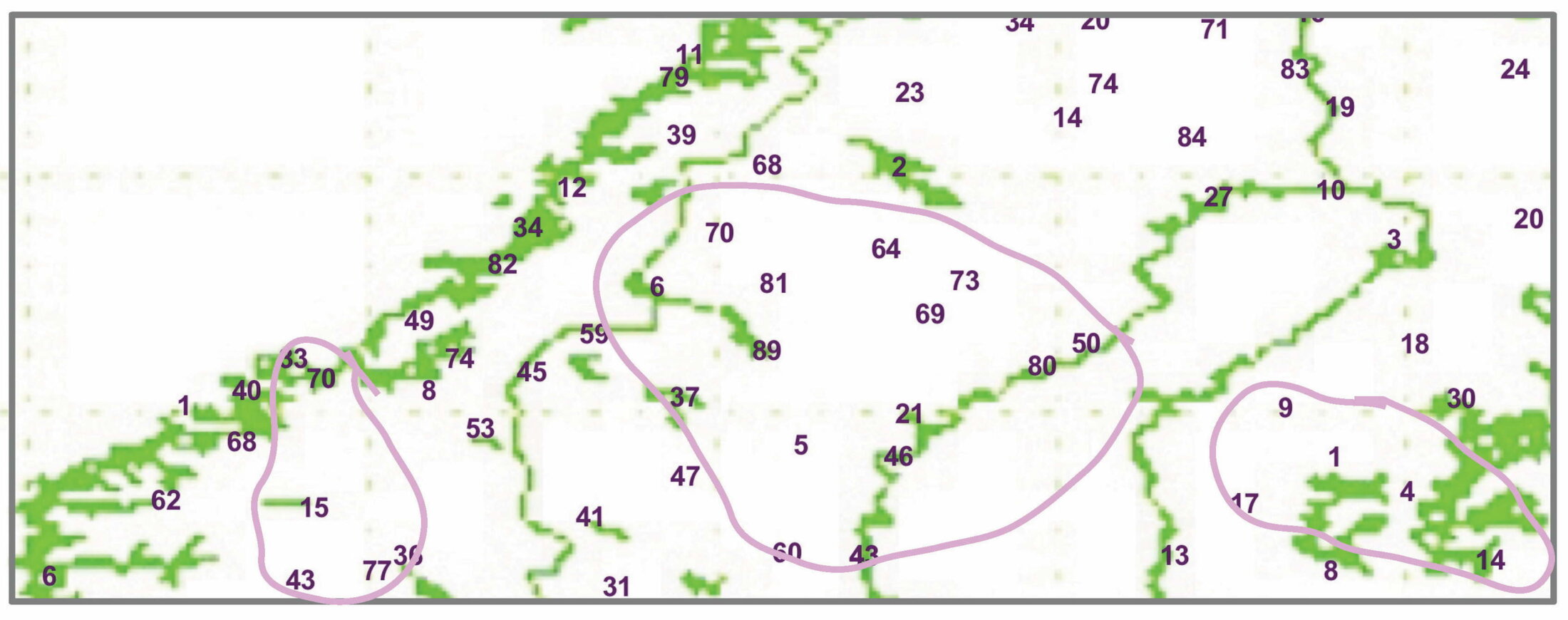
Scandinavia, beyond latitude 60.5 degrees North
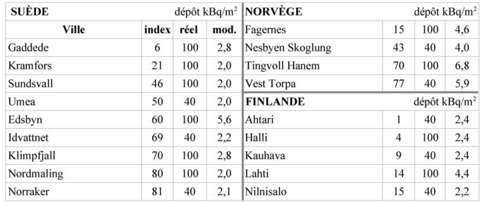
Agrandissement : Illustration 12
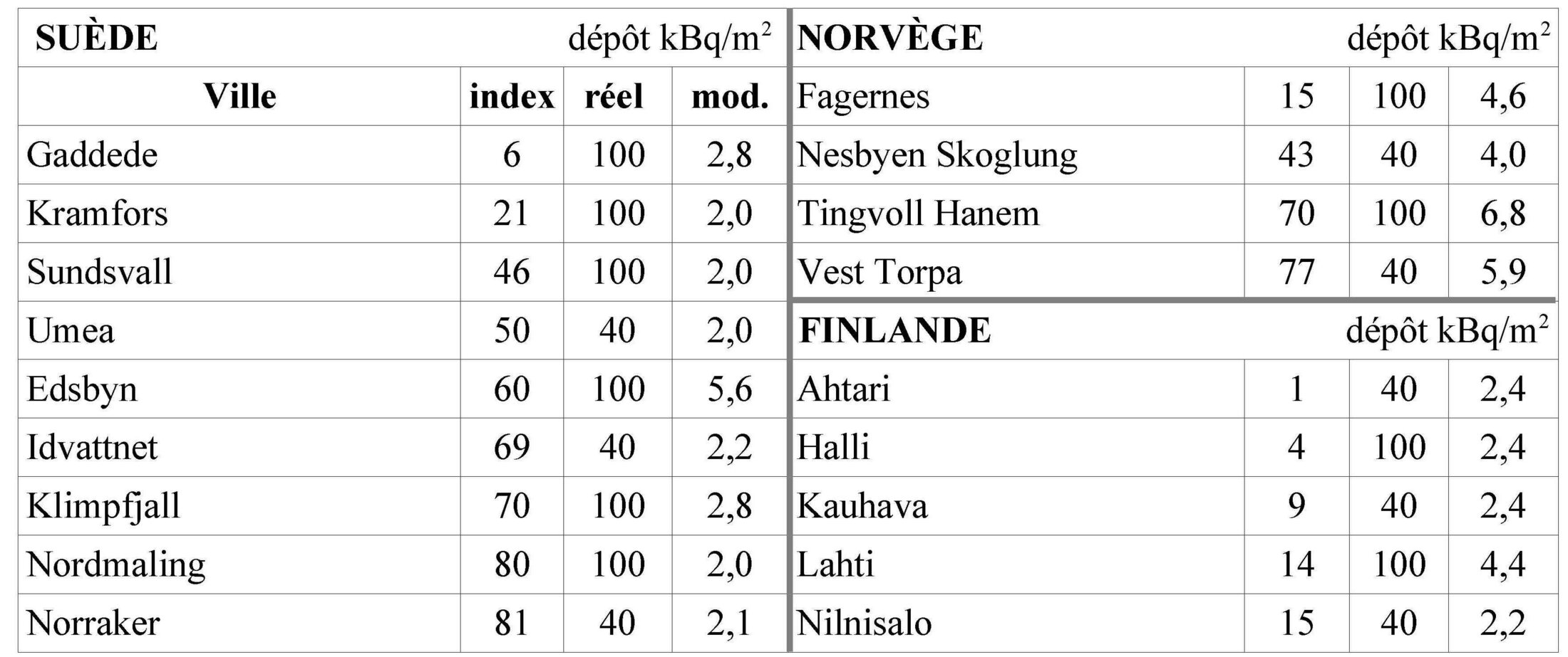
List of cities that experienced significant radioactive fallout from 10 to 12 May 1986
3.7. The deposition on Russia shows an arc of very high values south of Moscow.

Agrandissement : Illustration 13
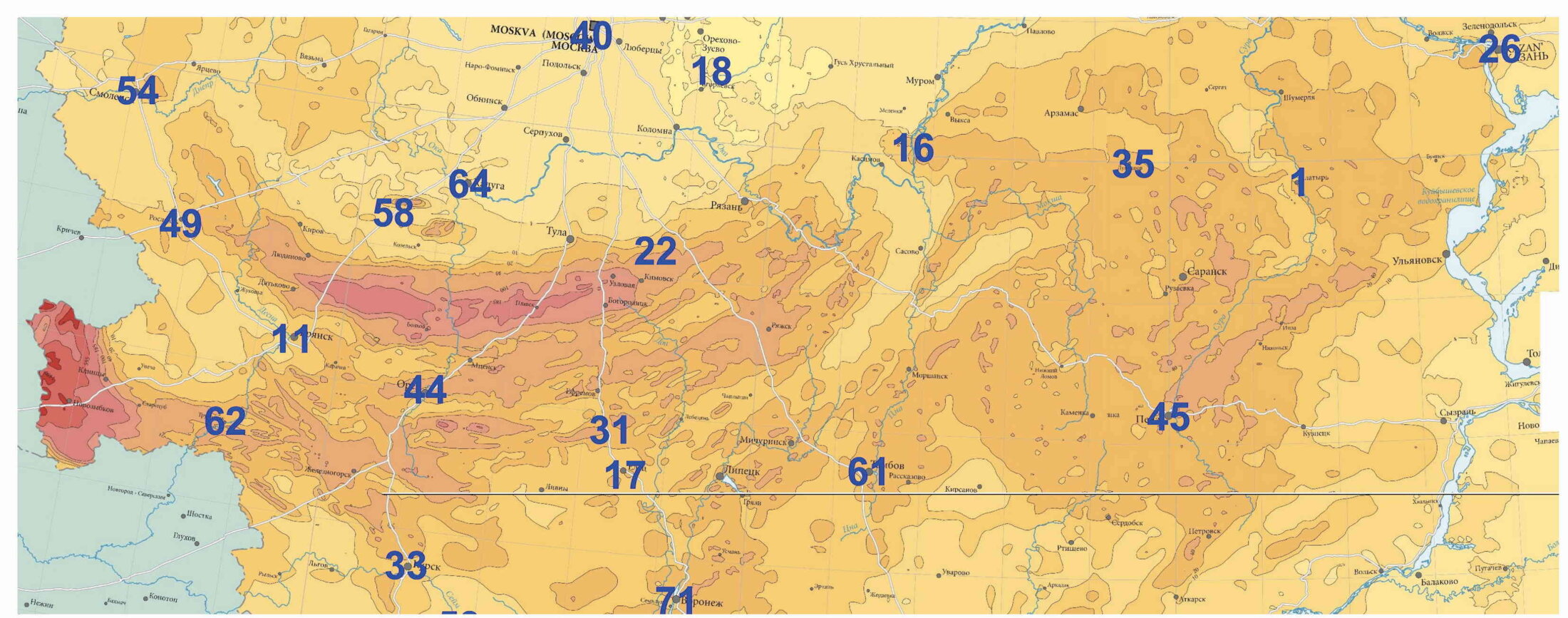
All Russian stations affected by the monitoring of radioactive fallout from Chernobyl
In her book Manual for Survival115, Kate Brown devotes five pages to the question of weather manipulation through the dispersion of AgI in a Chernobyl plume. She refers to a report presented in 2006 to the Central Committee of the Republic of Belarus by the chief authorising officer of these operations, Youry Izrael. In 1986, Y. Izrael was the head of the USSR State Committee for Hydrometeorology and headed the Liquidation Commission, one of whose missions was to maintain absolute secrecy on everything related to the management of the Chernobyl crisis. The information disclosed may be incomplete. Contrary to what she wrote, Voronezh [71] suffered a much greater fallout than that reconstructed with the IRSN model: 40 kBq/m2 compared with 2.6. The map above shows that the most contaminated area escapes analysis because no meteorological station is included. For the others, the data suggest a determination to continue plumes seeding after the initial major purge.
Indeed, as the logarithmic graph shows, only the following stations (indexed here according to the map) are not outside the [-0.5 ; +0.5] range: Trubcevsk [62], Kaluga [64], Orel [44] and Ielets [17]. The other twelve most likely received provoked fallout or some unexpected slag: Smolensk [54], Roslavi [49], Suhinici [58], Kursk [33], Jeti-Konur [22], Krasno-Scekovo [31], Voronezh [71], Elat'ma [16], Tambov [61], Lukojanov [35], Penza [45] and Alatyr [1].
It is true that the wind was turning, the rainfall forecast was still uncertain. Prevention was preferred to cure - evacuating and decontaminating large cities16. No soothing speech like those that abused world opinion would have resisted the evacuation of a large city, especially if it was more than 300 or 400 km from the power station. Agricultural regions were sacrificed, both in Russia and in Belarus and the Ukraine, with most of their inhabitants....
An unanswered question remains: was it the quality of the spotting and the skill of the crews responsible for sowing the radioactive plumes, or luck, which avoided the worst in Gomel and Moghilev? For their immediate surroundings are almost as polluted as the Braghin and Khoïniki region, on the borders of the power station's "exclusion zone".
4. Teachings
This empirical and experimental work enriches and corrects the rare published information on the control of Chernobyl fallout. The speed with which it was implemented from the start of the crisis reveals the existence of plans, no doubt designed for the conduct of an atomic war, but also the immediate availability of an airborne force specially prepared for this type of intervention17.
The rather exceptional success of the operations was the key to the success of the Kremlin's communication strategy. By precipitating and dispersing a maximum amount of radioactivity over sparsely populated countryside, thanks to a secret strictly respected by the Liquidation Commission and the ban on disseminating any information whatsoever on the health damage among the first cohorts of liquidators (essentially military personnel), the crisis managers were able to avoid the outbreak of uncontrollable panic and the revelation of the human cost of liquidating the accident before it was over. In this respect, nothing of the unprecedented scale of the human damage (apart from the selected heroes, 28 firefighters) is reflected in the official report presented on behalf of the Soviet government by academician Valery Legasov to the IAEA Conference in Vienna in August 1986. The tone was set and priority was and remains given to the technical aspects of the Chernobyl war.
Another lesson: the almost total absence of thyroid pathologies among the Polish population is rather the result of the absence of rainfall while the country was under the Chernobyl plume, and less of the distribution of iodine tablets whose protective action does not exceed a few days, less than the radioactive period of I131. The purges carried out in Ukraine and Belarus contributed somewhat to this favourable outcome.
But it should be stressed here that it is not the passage of a radioactive cloud that causes the most damage to health; it is the fallout entering the food chain. The Corsican example is very instructive in this respect: the majority of the families of shepherds who consumed the milk and cheese produced by their farms suffered from the fallout from Chernobyl.
Finally, it is well understood that no country that has not seriously prepared for atomic war can actively confront a large-scale nuclear accident and reduce its most devastating consequences in the short and medium term. It can only suffer it, like Japan after Fukushima.
Notes
1 <https://www.irsn.fr/FR/popup/Pages/tchernobyl_video_nuage.aspx>
3 <https://fr.tutiempo.net/climat/europe.html>
et, exemple, <https://www.meteociel.fr/climatologie/obs_villes.php?code=33041&mois=4&annee=1986>
4 Head of Enfants de Tchernobyl Belarus, author of La Comédie Atomique, La Découverte, 2016 and, withMarc Petitjean, of the movieTchernobyl, le Monde d'Après, ETB, 2018.
5 The establishment of the file was coordinated by Youry Izrael, head of the Liquidation Commission established after the accident. As head of the USSR Hydrometeorological Service, it is unlikely that he did not supervise the monitoring of the fallout...
6 <http://www.aec.go.jp/jicst/NC/sitemap/pdf/P-4.pdf>
7 Belarus : 3 ; Lithuania : 1 ; Sweden : 12 ; Norway : 5 ; Finland : 6 ; Poland : 5 ; Ukraina: 6 ; Russia : 13. Total : 51 from 360.
8 On 27 April 1988, I had carried out roadside cores at the northern exit of the town, which the CRIIRAD had analysed. I had been surprised by the result, an average of 40 kBq/m2 for the isotopes 137 and 134 of caesium. This value contradicted the panic scene relationships in the city during the passage of the Chernobyl cloud, between April 30 and May 5. It did not rain during this period according to the airport weather station. We will come back to this because, in the absence of rain, IRSN's simulation reproducing the deposition phenomena, the contamination should have been around 350 kBq/m2 at the time. The density of the cloud was therefore probably much lower. This will have repercussions on the deposition values measured downwind.
9 [36] index locating the city on the map; each country has its own index list; look for the city index in its country.
10 On the night of the following day, 28 April 1986, the physicist Vassily Nesterenko measured radioactivity 3,000 times higher than normal when he arrived in Braghin from Minsk (see his account <http://enfants-tchernobyl-belarus.org/doku.php?id=base_documentaire:articles-2003:etb-137>). Such a level is mainly due to the radioelements deposited on the ground, and to a lesser extent only to the density of the radioactive plume.
11 In Novozybkov, in April 1990, I measured a gamma background noise level between 3 and 7 µSv/h, 25 to 60 times the normal level. Moreover, a map of ß-radiation in the Bryansk oblast drawn up between 30 May and 13 June 1986, which I photographed in Moscow the following day, reveals deposits of between 1,480 and 9,250 kBq/m2 in the whole border region with Belarus. This is the major effect for Russia of the plume purge carried out on 28-29 April in the whole of this region.
12 Gomel narrowly escaped this purge: the deposit in the city increases from 40 to 100 kBq/m2 (theoretical deposit 90 kBq/m2), but grows spectacularly as soon as one moves northeast, from 100 to 1480 kBq/m2 in less than 15 km.
13 Against 296 and 185 kBq/m2respectively, depending on the model.
14 Against, depending on the model: 9.7 kBq/m2 in Roslavi; 3.3 kBq/m2 in Smolensk; 3.1 kBq/m2 in Suhinichi; 2.4 kBq/m2 in Jeti-Konur.
15 Allen Lane, Penguin Book, 2019.
16 At the end of the "arc" are Kazan with Tupolev factory 22 and Samara (factory 1)... at Voronezh, under the arc, factory 64 ...add: aviation factory in Saratov, ditto Ulyanovsk, Tambov (air base and Mitchourinsk, missile equipment), Tula (historical arms factory), Ryazan (major electronics industry), Nizhny Novgorod (major computer centre), Kaluga,(marine engines, aircraft engines, tank engines, military electronics).
17 It was and remains made up of Tupolev 16 RR bombers, carrying a laboratory for the analysis of air radioactivity and AgI dispersion equipment. The Soviet air force was and remains - Russian - equipped with 9 such aircraft.